pyGWRetrieval

A Python package for retrieving and analyzing USGS groundwater level data.

Overview

pyGWRetrieval simplifies the process of downloading USGS groundwater level data (field measurements, daily values, and instantaneous values) via the modern USGS Water Data API. It supports various spatial inputs including:

Zip codes with customizable buffer distances
GeoJSON files for custom areas of interest
Shapefiles including state boundaries or groundwater basins
Point vectors with buffer capabilities
Polygon features for direct spatial queries

Features

🌍 Flexible Spatial Inputs: Query by zip code, GeoJSON, shapefile, or specific site numbers
� Multiple Data Sources: Retrieve from gwlevels, daily values, or instantaneous values
📊 Temporal Aggregation: Aggregate data to monthly, annual, growing season, or custom periods
📈 Visualization: Built-in plotting for time series analysis
💾 Multiple Export Formats: Save data as CSV or Parquet files
🔧 Trend Analysis: Calculate linear trends for water level changes
🗺️ Water-Table Depth Maps: Interpolate point observations to gridded rasters (IDW, kriging, RBF, linear, nearest) at a resolution you set in meters
💧 Aquifer Filtering: Retrieve aquifer type and restrict to unconfined (water-table) wells
⚡ Parallel Processing: Dask-powered parallel processing for large datasets
🌐 Modern USGS API: Built on the USGS Water Data OGC API with native large-area request chunking

USGS Data Sources

pyGWRetrieval supports three USGS NWIS data sources for groundwater levels:

Source	Description	Typical Use Case
`gwlevels`	Field groundwater-level measurements - Discrete manual measurements taken during field visits. Most accurate but infrequent.	Long-term trend analysis, calibration
`dv`	Daily values - Daily statistical summaries (mean, min, max) computed from continuous sensors.	Regular monitoring, daily patterns
`iv`	Instantaneous values - Current/historical observations at 15-60 minute intervals from continuous sensors.	High-resolution analysis, recent conditions

Selecting Data Sources

from pyGWRetrieval import GroundwaterRetrieval

# Default: dv (daily values)
gw = GroundwaterRetrieval(start_date='2020-01-01')
data = gw.get_data_by_zipcode('89701', buffer_miles=10)

# All available sources
gw_all = GroundwaterRetrieval(
    start_date='2020-01-01',
    data_sources='all'  # gwlevels + dv + iv
)

# Specific sources
gw_daily = GroundwaterRetrieval(
    start_date='2020-01-01',
    data_sources=['gwlevels', 'dv']  # Field measurements + daily values
)

# Single source
gw_instant = GroundwaterRetrieval(
    start_date='2020-01-01',
    data_sources='iv'  # Instantaneous values only
)

The output data includes a data_source column to identify which source each record came from.

Note on Data Aggregation: All three data types (gwlevels, dv, iv) are stored as-is after download without any aggregation or transformation. Daily values (dv) are pre-computed by USGS, and instantaneous values (iv) retain their original high-frequency resolution (typically 15-60 minute intervals). If you need to aggregate iv data to daily or other frequencies, use the TemporalAggregator class from the temporal module.

Data backend: As of v0.2.0, pyGWRetrieval uses the modern USGS Water Data OGC API (dataretrieval >= 1.2.0, the waterdata module) for all retrieval — get_monitoring_locations, get_daily, get_continuous, and get_field_measurements. This restores gwlevels field-measurement retrieval (the deprecated NWIS endpoint returned an HTML notice instead of data) and adds native large-area request chunking. The legacy NWIS endpoints are kept only as an automatic fallback. Note that site_no now carries the full monitoring-location id (e.g. USGS-393000119000001).

Installation

Using pip

pip install pyGWRetrieval

From source

git clone https://github.com/montimaj/pyGWRetrieval.git
cd pyGWRetrieval
pip install -e .

With optional dependencies

# For enhanced visualization
pip install pyGWRetrieval[viz]

# For distributed computing (multi-node parallelism)
pip install pyGWRetrieval[distributed]

# For development
pip install pyGWRetrieval[dev]

# For documentation
pip install pyGWRetrieval[docs]

# All optional dependencies
pip install pyGWRetrieval[all]

Project Structure

pyGWRetrieval/
├── pyGWRetrieval/           # Main package
│   ├── __init__.py          # Package initialization and exports
│   ├── retrieval.py         # Core GroundwaterRetrieval class
│   ├── spatial.py           # Spatial utilities (zip codes, geometries, buffers)
│   ├── temporal.py          # Temporal aggregation and trend analysis
│   ├── interpolation.py     # Water-table depth interpolation
│   ├── visualization.py     # Plotting and visualization tools
│   ├── parallel.py          # Dask-based parallel processing
│   ├── cli.py               # Command-line interface
│   └── utils.py             # Helper functions and utilities
├── docs/                    # Documentation (MkDocs)
│   ├── index.md             # Documentation home
│   ├── quickstart.md        # Getting started guide
│   ├── interpolation.md     # Interpolation guide
│   ├── api_reference.md     # API documentation
│   └── cli.md               # CLI documentation
├── examples/                # Example sets (each with its own README)
│   ├── ucrc/                # Upper Colorado Basin water-table depth mapping
│   └── msa_analysis/        # 9-MSA case study + general usage scripts
├── tests/                   # Unit tests
├── pyproject.toml           # Package configuration
├── setup.py                 # Setup script
├── requirements.txt         # Dependencies
├── LICENSE                  # MIT License
└── README.md                # This file

Quick Start

Basic Usage

from pyGWRetrieval import GroundwaterRetrieval

# Initialize with date range
gw = GroundwaterRetrieval(
    start_date='2010-01-01',
    end_date='2023-12-31'
)

# Get data by zip code with 10-mile buffer
data = gw.get_data_by_zipcode('89701', buffer_miles=10)

# Save to CSV
gw.to_csv('groundwater_data.csv')

Using Multiple Zip Codes from CSV

from pyGWRetrieval import GroundwaterRetrieval

gw = GroundwaterRetrieval()

# Read zip codes from CSV file - parallel processing is enabled by default
data = gw.get_data_by_zipcodes_csv(
    'locations.csv',
    zipcode_column='zip',  # Name of column with zip codes
    buffer_miles=10,
    parallel=True,         # Enable parallel processing (default)
    n_workers=4            # Optional: specify number of workers
)

# Results include 'source_zipcode' column to track origin
print(data['source_zipcode'].value_counts())

# Save data to separate files per zip code
saved_files = gw.save_data_per_zipcode('output_by_zipcode/', file_format='csv')
for zipcode, filepath in saved_files.items():
    print(f"Saved {zipcode} to {filepath}")

Using Shapefiles

from pyGWRetrieval import GroundwaterRetrieval

gw = GroundwaterRetrieval()

# Get data within a polygon (e.g., basin boundary)
data = gw.get_data_by_shapefile('my_basin.shp')

# For point shapefiles, specify a buffer
data = gw.get_data_by_shapefile('well_locations.shp', buffer_miles=5)

Large areas (new in v0.2.0): Queries over whole hydrologic regions or large basins work with no extra configuration — the USGS Water Data OGC API chunks large bounding-box requests natively, and results are clipped to the requested geometry. (If the deprecated NWIS fallback is ever used, its 25-square-degree bBox limit is handled by automatic sub-box tiling.) See the examples README for an Upper Colorado River Basin example.

Example: Monthly water levels for the Upper Colorado River Basin

The examples/ucrc/ directory ships a basin polygon (UCRB_WBDHU2, WBD HU2 = 14). Its bounding box spans ~53 square degrees, so the query is automatically chunked. The snippet below downloads the latest 5 years of daily values (dv, the default source) for the basin and aggregates them to monthly mean water levels:

from pyGWRetrieval import GroundwaterRetrieval, TemporalAggregator

# Default source is 'dv' (daily values); the oversized basin bbox is
# auto-chunked and wells are clipped to the polygon.
gw = GroundwaterRetrieval(start_date='2021-07-08', end_date='2026-07-08')
data = gw.get_data_by_shapefile('examples/ucrc/UCRB_WBDHU2/UCRB_WBDHU2.shp')

# Wells report different USGS parameters. Each record's parameter is exposed
# in the 'parameter_cd' column, so filter to depth-to-water (72019, feet below
# land surface) to keep every well on the same footing.
depth = data[data['parameter_cd'] == '72019']

# Monthly mean depth-to-water per well (dv uses the 'datetime' date column).
aggregator = TemporalAggregator(depth, date_column='datetime', value_column='lev_va')
monthly = aggregator.to_monthly(agg_func='mean')

monthly.to_csv('ucrb_monthly_gwl.csv', index=False)
print(f"{len(monthly)} monthly records from {depth['site_no'].nunique()} wells")

A runnable version is provided as examples/ucrc/retrieve_ucrb.py.

Using GeoJSON

from pyGWRetrieval import GroundwaterRetrieval

gw = GroundwaterRetrieval(start_date='2020-01-01')

# Get data within GeoJSON polygons
data = gw.get_data_by_geojson('study_area.geojson')

# Save as Parquet
gw.to_parquet('groundwater_data.parquet')

Temporal Aggregation

from pyGWRetrieval import GroundwaterRetrieval, TemporalAggregator

# Get raw data
gw = GroundwaterRetrieval()
data = gw.get_data_by_zipcode('89701', buffer_miles=20)

# Aggregate temporally
aggregator = TemporalAggregator(data)

# Monthly means
monthly = aggregator.to_monthly(agg_func='mean')

# Annual medians
annual = aggregator.to_annual(agg_func='median')

# Growing season (April-September)
growing = aggregator.to_growing_season(start_month=4, end_month=9)

# Water year
water_year = aggregator.to_annual(water_year=True)

# Custom period (e.g., summer months)
summer = aggregator.to_custom_period(months=[6, 7, 8], period_name='summer')

Water-Table Depth Maps (Spatial Interpolation)

Turn point observations into gridded water-table depth maps for a chosen window ('all', 'monthly', 'annual', or 'custom') at a resolution you specify in meters. Supported methods: idw (inverse distance weighting), kriging (ordinary), and linear / cubic / nearest / rbf. Requires the interp extra (pip install pyGWRetrieval[interp]) for kriging and the scipy-based methods; IDW works with the core install.

from pyGWRetrieval import GroundwaterRetrieval, WaterTableInterpolator
from pyGWRetrieval.spatial import get_geometry_from_shapefile, merge_geometries

# Field measurements + daily values for a basin, 1985-present.
gw = GroundwaterRetrieval(start_date='1985-01-01', data_sources=['gwlevels', 'dv'])
data = gw.get_data_by_shapefile('basin.shp')

# Keep depth-to-water (param 72019) at UNCONFINED wells only — water-table
# depth is only meaningful for unconfined aquifers. Discovery already attached
# aqfr_type_cd to gw.wells.
depth = data[data['parameter_cd'] == '72019']
unconfined = set(gw.wells.loc[gw.wells['aqfr_type_cd'] == 'U', 'site_no'])
wtd = depth[depth['site_no'].isin(unconfined)]

# Long-term mean water-table depth on a 1 km grid, clipped to the basin.
basin = merge_geometries(get_geometry_from_shapefile('basin.shp'))
interp = WaterTableInterpolator(wtd, value_column='lev_va', date_column='datetime')
grids = interp.interpolate(period='all', method='idw', grid_size_m=1000, boundary=basin)

result = grids['all']
result.to_geotiff('wtd_mean_idw.tif')   # also .plot() and .to_xarray()

interpolate() returns a dict of window label → InterpolationResult, each of which supports .plot(), .to_geotiff(), and .to_xarray().

The Upper Colorado River Basin example builds a long-term mean water-table depth map (1985-present) and compares five interpolation methods on the same 1 km grid. It uses the 496 confirmed unconfined wells as a reference and, rather than discarding the unclassified/mixed wells, keeps those whose mean depth-to-water is consistent with the unconfined water-table surface (within its leave-one-out variability, via idw_at_points) — 1,120 wells in total. See the examples README for the full walkthrough (data funnel, gap-fill, and a threshold-sensitivity comparison).

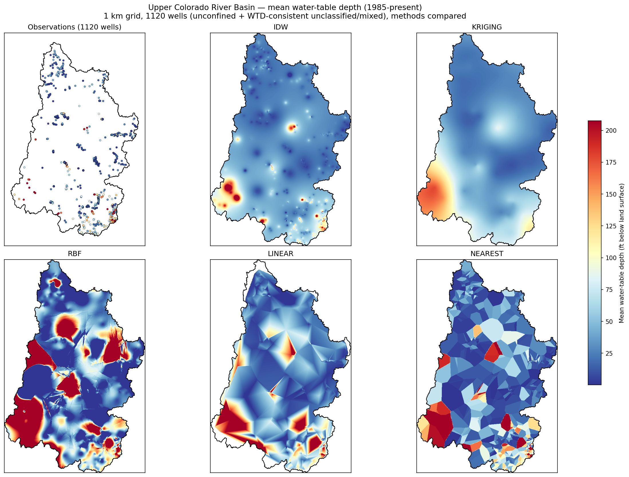
The panels highlight the methods' characteristics: IDW produces smooth "bullseyes" around wells, Kriging gives a smooth geostatistical surface, RBF (thin-plate spline) fits observations tightly but overshoots when extrapolating beyond the data, Linear only fills the Delaunay convex hull of the points (it does not extrapolate, so cells beyond the hull are left blank), and Nearest yields hard Voronoi cells. Grid resolution is set in meters (grid_size_m); observations are projected to a metric CRS (auto-UTM by default) before interpolation.

To give linear/cubic full basin coverage, pass fill_outside='nearest' (or 'idw') — cells the primary method leaves empty are backfilled by the secondary method:

interp.interpolate(period='all', method='linear', grid_size_m=1000,
                   boundary=basin, fill_outside='nearest')

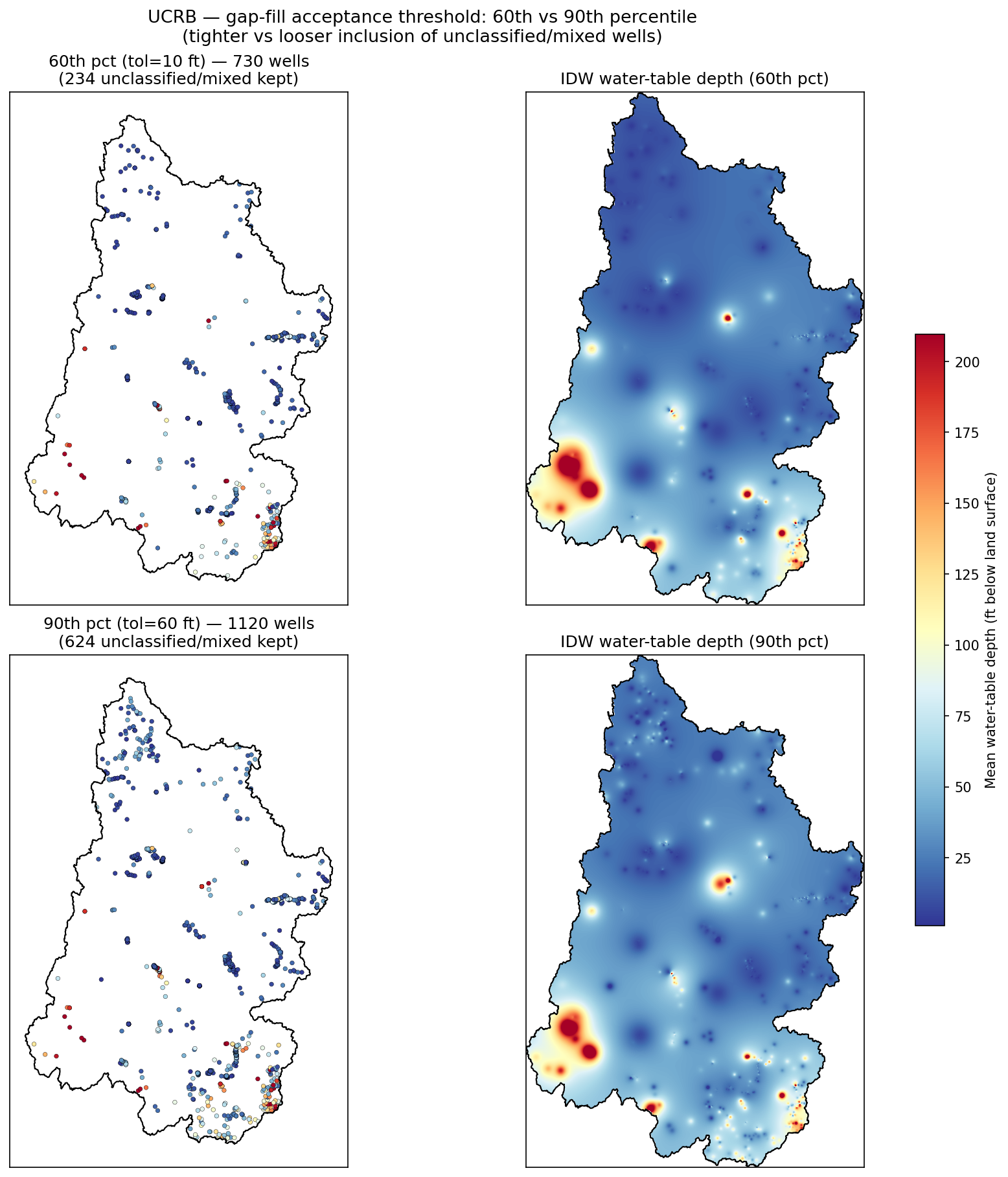
Sensitivity to the well set. The example gap-fills unclassified/mixed wells by keeping only those consistent with the unconfined water-table surface; how inclusive that is depends on an acceptance band (--consistency-pct). A tighter band (60th percentile, 730 wells) vs a looser one (90th percentile, 1,120 wells) mostly changes coverage in data-sparse areas — the regional pattern is stable:

Tip: choose a resolution appropriate for your well density and extent. A very fine grid over a large, sparsely-monitored basin (e.g. 30 m over the ~293,000 km² Upper Colorado Region — hundreds of billions of cells) is neither tractable nor statistically meaningful.

Visualization

from pyGWRetrieval import GroundwaterRetrieval, GroundwaterPlotter
import matplotlib.pyplot as plt

# Get data
gw = GroundwaterRetrieval()
data = gw.get_data_by_zipcode('89701', buffer_miles=15)

# Create plotter
plotter = GroundwaterPlotter(data)

# Time series for all wells
fig = plotter.plot_time_series()
plt.savefig('time_series.png')

# Single well detailed plot
fig = plotter.plot_single_well('390000119000001')
plt.savefig('single_well.png')

# Monthly boxplot
fig = plotter.plot_monthly_boxplot()
plt.savefig('monthly_boxplot.png')

# Annual summary
fig = plotter.plot_annual_summary()
plt.savefig('annual_summary.png')

Spatial Map Visualization

Create maps showing wells colored by water level with automatic zoom:

from pyGWRetrieval import GroundwaterRetrieval, plot_wells_map, create_comparison_map
import matplotlib.pyplot as plt

# Get data from multiple zip codes
gw = GroundwaterRetrieval()
data = gw.get_data_by_zipcodes_csv('locations.csv', zipcode_column='zip', buffer_miles=20)

# Create a spatial map with auto-zoom
# - Local extent (<20 mi): detailed zoom
# - Regional extent (<100 mi): wider view
# - State extent (<500 mi): state-level view
# - National extent (>1500 mi): continental view
fig = plot_wells_map(
    data,
    agg_func='mean',  # Show mean water level per well
    title='Groundwater Wells (ft below surface)',
    cmap='RdYlBu_r',  # Red=deep water, Blue=shallow
    add_basemap=True,  # Add OpenStreetMap-style basemap
    group_by_column='source_zipcode'  # Label by zip code
)
plt.savefig('wells_map.png', dpi=300)

# Create a 4-panel comparison map (mean, min, max, record count)
fig = create_comparison_map(data, figsize=(18, 12))
plt.savefig('comparison_map.png', dpi=300)

Parallel Processing

pyGWRetrieval uses Dask for parallel processing of large datasets:

from pyGWRetrieval import GroundwaterRetrieval, check_dask_available, get_parallel_config

# Check if parallel processing is available
print(f"Dask available: {check_dask_available()}")
print(f"Config: {get_parallel_config()}")

# Parallel processing is enabled by default for multi-zipcode queries
gw = GroundwaterRetrieval(start_date='1970-01-01')
data = gw.get_data_by_zipcodes_csv(
    'locations.csv',
    zipcode_column='zip',
    parallel=True,           # Default
    n_workers=4,             # Number of parallel workers
    scheduler='threads'      # 'threads', 'processes', or 'synchronous'
)

# For distributed computing across multiple machines
from pyGWRetrieval import get_dask_client

client = get_dask_client(n_workers=8)  # Creates local cluster
# Dashboard available at client.dashboard_link

Command Line Interface (CLI)

pyGWRetrieval provides a full-featured CLI for all operations.

Installation

After installing the package, the pygwretrieval command is available:

pygwretrieval --help

Retrieve Data

# By zip code with buffer (default: dv / daily values)
pygwretrieval retrieve --zipcode 89701 --buffer 10 --output data.csv

# Retrieve from all USGS data sources (gwlevels, dv, iv)
pygwretrieval retrieve --zipcode 89701 --buffer 10 --data-sources all --output data.csv

# Retrieve from specific sources
pygwretrieval retrieve --zipcode 89701 --data-sources gwlevels dv --output data.csv

# From CSV file with multiple zip codes (parallel processing)
pygwretrieval retrieve --csv locations.csv --zipcode-column zip --parallel --output data.csv

# Multi-source retrieval from CSV
pygwretrieval retrieve --csv locations.csv --zipcode-column zip --data-sources all --parallel --output data.csv

# Save separate files per zip code
pygwretrieval retrieve --csv locations.csv --zipcode-column zip --save-per-zipcode --per-zipcode-dir output/

# From shapefile
pygwretrieval retrieve --shapefile basin.shp --buffer 5 --output basin_data.csv

# From GeoJSON
pygwretrieval retrieve --geojson study_area.geojson --output area_data.csv

# By state
pygwretrieval retrieve --state NV --output nevada_data.csv

# Specific sites
pygwretrieval retrieve --sites 390000119000001 390000119000002 --output sites_data.csv

# With date range
pygwretrieval retrieve --zipcode 89701 --start-date 2010-01-01 --end-date 2023-12-31 --output data.csv

# Save well locations as GeoJSON
pygwretrieval retrieve --zipcode 89701 --buffer 15 --output data.csv --wells-output wells.geojson

Aggregate Data

# Monthly aggregation
pygwretrieval aggregate --input data.csv --period monthly --output monthly.csv

# Annual aggregation
pygwretrieval aggregate --input data.csv --period annual --agg-func mean --output annual.csv

# Water year aggregation
pygwretrieval aggregate --input data.csv --period water-year --output water_year.csv

# Growing season (April-September)
pygwretrieval aggregate --input data.csv --period growing-season --start-month 4 --end-month 9 --output growing.csv

# Custom period with median
pygwretrieval aggregate --input data.csv --period custom --start-month 6 --end-month 8 --agg-func median --output summer.csv

Calculate Statistics and Trends

# Both statistics and trends
pygwretrieval stats --input data.csv --output analysis

# Statistics only
pygwretrieval stats --input data.csv --output stats --type statistics

# Trends with parallel processing
pygwretrieval stats --input data.csv --output trends --type trends --parallel

Create Visualizations

# Time series plot
pygwretrieval plot --input data.csv --type timeseries --output timeseries.png

# Single well detailed plot with trend
pygwretrieval plot --input data.csv --type single-well --wells 390000119000001 --show-trend --output well.png

# Monthly boxplot
pygwretrieval plot --input data.csv --type boxplot --output boxplot.png

# Annual summary
pygwretrieval plot --input data.csv --type annual --output annual.png

# Custom figure size and DPI
pygwretrieval plot --input data.csv --type timeseries --figsize 14 10 --dpi 300 --output plot.png

Create Spatial Maps

# Basic map with basemap
pygwretrieval map --input data.csv --output wells_map.png --basemap

# Map with custom colormap and grouping
pygwretrieval map --input data.csv --output map.png --basemap --cmap viridis --group-by source_zipcode

# Different basemap provider
pygwretrieval map --input data.csv --output map.png --basemap --basemap-source Esri.WorldImagery

# Comparison map (4 panels: mean, count, min, max)
pygwretrieval map --input data.csv --output comparison.png --comparison --basemap

Get Data Information

# Basic info
pygwretrieval info --input data.csv

# Detailed statistics
pygwretrieval info --input data.csv --detailed

Global Options

# Verbose output
pygwretrieval -v retrieve --zipcode 89701 --output data.csv

# Quiet mode (errors only)
pygwretrieval -q retrieve --zipcode 89701 --output data.csv

# Version
pygwretrieval --version

API Reference

Core Classes

`GroundwaterRetrieval`

Main class for data retrieval from the USGS Water Data API.

GroundwaterRetrieval(start_date='1900-01-01', end_date=None, data_sources='dv')

Parameters:

start_date (str): Start date in 'YYYY-MM-DD' format (default: '1900-01-01')
end_date (str): End date (default: today)
data_sources (str | List): Data sources to retrieve:
- 'dv' (default): Daily values
- 'gwlevels': Field measurements
- 'iv': Instantaneous values
- 'all': All sources
- ['gwlevels', 'dv']: List of specific sources

Methods:

get_data_by_zipcode(zipcode, buffer_miles, country) - Query by zip code
get_data_by_zipcodes_csv(filepath, zipcode_column, buffer_miles) - Query multiple zip codes from CSV
get_data_by_geojson(filepath, buffer_miles, layer) - Query using GeoJSON
get_data_by_shapefile(filepath, buffer_miles) - Query using shapefile
get_data_by_state(state_code) - Query entire state
get_data_by_sites(site_numbers) - Query specific sites
get_aquifer_info(site_numbers, merge) - Retrieve aquifer type (aqfr_type_cd) and attributes
to_csv(filepath) - Export to CSV
to_parquet(filepath) - Export to Parquet
save_data_per_zipcode(output_dir, file_format, prefix) - Save data per zip code

`WaterTableInterpolator`

Interpolate point water levels to gridded water-table depth maps.

WaterTableInterpolator(data, value_column='lev_va', site_column='site_no',
                       date_column='datetime', lat_column='dec_lat_va',
                       lon_column='dec_long_va', crs='EPSG:4326')

Methods:

interpolate(period, method, grid_size_m, boundary, ...) - Returns {window: InterpolationResult}. period ∈ {'all','monthly','annual','custom'}; method ∈ {'idw','kriging','linear','cubic','nearest','rbf'}; grid_size_m sets the cell size in meters.

Each InterpolationResult has .grid, .x, .y, .crs and methods .plot(), .to_geotiff(path), .to_xarray().

`TemporalAggregator`

Class for temporal aggregation of groundwater data.

TemporalAggregator(data, date_column='lev_dt', value_column='lev_va', site_column='site_no')

Methods:

to_monthly(agg_func, include_count) - Monthly aggregation
to_annual(agg_func, water_year) - Annual aggregation
to_growing_season(start_month, end_month, region) - Growing season aggregation
to_custom_period(months, period_name) - Custom period aggregation
to_weekly(agg_func) - Weekly aggregation
resample(freq, agg_func) - Pandas resample
calculate_statistics(groupby) - Comprehensive statistics
get_trends(period) - Linear trend analysis

`GroundwaterPlotter`

Class for visualization of groundwater data.

GroundwaterPlotter(data, date_column='lev_dt', value_column='lev_va', site_column='site_no')

Methods:

plot_time_series(wells, figsize, title) - Time series plots
plot_single_well(site_no, show_trend, show_stats) - Detailed single well plot
plot_comparison(wells, normalize) - Multi-well comparison
plot_monthly_boxplot(wells) - Monthly distribution
plot_annual_summary(wells, agg_func) - Annual statistics
plot_heatmap(well, cmap) - Year-month heatmap
plot_spatial_distribution(wells_gdf) - Spatial map

Utility Functions

from pyGWRetrieval import (
    save_to_csv,
    save_to_parquet,
    validate_date_range,
    setup_logging,
)

# Configure logging
setup_logging(level=logging.DEBUG, log_file='pyGWRetrieval.log')

Data Sources

This package retrieves USGS groundwater data via the modern USGS Water Data OGC API (with the legacy National Water Information System, NWIS, kept as an automatic fallback), using the dataretrieval-python library (≥ 1.2.0).

Available Data Sources

Source	API Function	Description	Use Case
`gwlevels`	`get_gwlevels()`	Field measurements - Discrete manual readings during field visits	Long-term trends, calibration
`dv`	`get_dv()`	Daily values - Daily statistical summaries from continuous sensors	Regular monitoring
`iv`	`get_iv()`	Instantaneous values - High-frequency (15-60 min) sensor data	Real-time analysis

USGS Parameter Codes

The following parameter codes are used for groundwater levels:

72019: Depth to water level, feet below land surface
72020: Elevation above NGVD 1929, feet
62610: Groundwater level above NGVD 1929, feet
62611: Groundwater level above NAVD 1988, feet

Site Type: GW (Groundwater)

Data Columns and Units

The package retrieves groundwater level data with the following columns:

Column	Description	Units
`site_no`	Monitoring location id (e.g. `USGS-393000119000001`)	-
`datetime`	Date/time of measurement (tz-naive)	datetime
`lev_dt`	Alias of `datetime`	datetime
`value`	Standardized water level value	Depends on `parameter_cd`
`lev_va`	Alias of `value`	Depends on `parameter_cd`
`parameter_cd`	USGS parameter code the value came from (e.g. `72019` depth-to-water, `62611` elevation)	-
`data_source`	Origin of the record (`gwlevels`, `dv`, or `iv`)	-
`unit_of_measure`	Unit reported by USGS (e.g. `ft`)	-
`approval_status`	Approval status of the value	-
`qualifier`	Data qualifier code(s)	-
`station_nm`	Station name (merged from site info)	-
`dec_lat_va`	Decimal latitude	Degrees
`dec_long_va`	Decimal longitude	Degrees
`source_zipcode`	Source zip code (for CSV queries)	-

The Water Data OGC API returns depth-to-water (parameter 72019) as feet below land surface; elevation parameters (62610/62611) are in feet relative to a vertical datum. Filter on parameter_cd to keep a single quantity. Additional monitoring-location attributes (e.g. aqfr_type_cd, alt_va) are attached to the wells GeoDataFrame.

USGS Parameter Codes

Code	Description	Units
`72019`	Depth to water level below land surface	Feet
`72020`	Elevation above NGVD 1929	Feet
`62610`	Groundwater level above NGVD 1929	Feet
`62611`	Groundwater level above NAVD 1988	Feet

Note: The primary measurement lev_va represents depth to water in feet below land surface. Lower values indicate a shallower water table, while higher values indicate deeper groundwater.

Requirements

Python ≥ 3.10
dataretrieval ≥ 1.2.0 (modern USGS Water Data OGC API)
pandas ≥ 1.3.0
geopandas ≥ 0.10.0
shapely ≥ 1.8.0
pyproj ≥ 3.0.0
pgeocode ≥ 0.3.0
matplotlib ≥ 3.4.0
numpy ≥ 1.20.0

Optional Dependencies

seaborn (enhanced visualizations)
contextily (basemaps for spatial plots)
pyarrow (Parquet support)
scipy (trend analysis; linear/cubic/nearest/rbf interpolation)
pykrige (ordinary kriging interpolation)
rasterio, xarray (GeoTIFF / xarray export of interpolated grids)

Install the interpolation stack with pip install pyGWRetrieval[interp].

Optional: USGS API Token

No API key is required — the USGS Water Data OGC API (and the legacy NWIS fallback) serve public data anonymously, so pyGWRetrieval works out of the box.

If you make heavy or frequent requests, you can optionally supply a USGS Personal Access Token (PAT) to raise the request rate limit. Request one from the USGS Water Data API. pyGWRetrieval relies on dataretrieval, which reads the token from the API_USGS_PAT environment variable and sends it as the X-Api-Key header on every request — no code or argument changes needed.

From the shell (applies to the CLI and Python):

export API_USGS_PAT="your-token-here"
pygwretrieval retrieve --state NV

From Python:

import os
os.environ["API_USGS_PAT"] = "your-token-here"  # must be set before making requests

from pyGWRetrieval import GroundwaterRetriever
gw = GroundwaterRetriever()
data = gw.get_data_by_state("NV")

The token only affects rate limits; all queries also work without it. Token support requires dataretrieval >= 1.2.0 (the version this package targets).

Storage Requirements

Storage requirements vary based on the number of zip codes, buffer distance, and data sources queried. Below are example estimates based on the full_workflow_csv_zipcodes.py example (99 zip codes, 25-mile buffer, gwlevels source, ~8M records):

Component	Size	Description
Combined Parquet	~80 MB	All retrieved groundwater data
Per-zipcode data	~130 MB	Individual parquet files per zip code
Wells GeoJSON	~25 MB	Well locations with metadata
Aggregated CSVs	~27 MB	Monthly and annual aggregations
Visualization plots	~15 MB	15 PNG figures at 300 DPI
Analysis CSVs	~2 MB	Trends, statistics, projections
Total	~275 MB	Complete workflow output

Scaling estimates:

~3 MB per 1,000 wells retrieved
~10 KB per groundwater measurement record (Parquet format)
Plot sizes: ~0.5-1.5 MB each at 300 DPI

Tip: Use Parquet format (default) for efficient storage. Parquet files are ~60% smaller than equivalent CSV files and load significantly faster.

Examples

The examples/ directory holds two self-contained example sets, each with its own README:

examples/ucrc/ — Upper Colorado River Basin: large-area retrieval, unconfined-aquifer filtering, and gridded water-table depth mapping with a five-method interpolation comparison.
examples/msa_analysis/ — Metropolitan analysis & general usage: a 9-MSA regional case study (full_workflow_csv_zipcodes.py) plus general scripts (basic_usage.py, temporal_analysis.py, advanced_spatial.py, multi_source_example.py).

Full Workflow Example

The full_workflow_csv_zipcodes.py demonstrates a complete pipeline:

from pyGWRetrieval import GroundwaterRetrieval, TemporalAggregator, GroundwaterPlotter

# 1. Read zip codes from CSV and download data from ALL USGS sources
gw = GroundwaterRetrieval(
    start_date='1970-01-01',
    data_sources='all'  # gwlevels + dv + iv
)
data = gw.get_data_by_zipcodes_csv(
    'locations.csv',
    zipcode_column='ZipCode',
    buffer_miles=100
)

# Data includes 'data_source' column identifying record origin
print(data.groupby('data_source').size())

# 2. Save combined and per-zipcode data
gw.to_csv('all_data.csv')
saved = gw.save_data_per_zipcode('output/', file_format='csv')

# 3. Temporal aggregation
aggregator = TemporalAggregator(data)
monthly = aggregator.to_monthly()
annual = aggregator.to_annual()

# 4. Visualization
plotter = GroundwaterPlotter(data)
fig = plotter.plot_time_series()

This workflow:

Processes multiple zip codes from a CSV file
Downloads historical groundwater data (1970-present)
Saves data both combined and per zip code
Performs monthly and annual aggregations
Creates time series, boxplot, and comparison visualizations

Case Study: Regional Groundwater Analysis of 9 U.S. Metropolitan Areas

The full_workflow_csv_zipcodes.py example demonstrates a comprehensive regional groundwater analysis across nine major U.S. Metropolitan Statistical Areas (MSAs): New York, Miami, Washington DC, Houston, Boston, Philadelphia, San Francisco, Chicago, and Dallas.

Note: this case study was produced with pyGWRetrieval v0.1.0. Results are substantially unchanged on the v0.2.0 Water Data OGC API backend.

Study Overview

Metric	Value
Total Records	7,995,927
Monitoring Wells	33,018
Temporal Coverage	1970-2025 (55 years)
Metropolitan Areas	9
Zip Codes Analyzed	99
Visualizations Generated	15 figures

Key Findings

Dallas shows remarkable groundwater recovery (+10.6 ft/year rising trend)
Washington DC is the only region with significant declining trend (+1.1 ft/year deepening)
Miami demonstrates the most stable groundwater conditions (lowest variability)
5 of 9 regions show statistically significant long-term trends (p < 0.05)

Generated Analyses

The workflow produces 15 publication-ready visualizations:

Regional Trends - Trend analysis by MSA
Data Quality - Coverage and density metrics
Distributions - Water level statistical distributions
Temporal Patterns - Decadal and seasonal patterns
Monthly/Annual Boxplots - Seasonal and inter-annual variability
Correlation & Clustering - Inter-regional relationships
Extreme Events - Drought and anomaly analysis
Rate of Change - Trend acceleration analysis
Geographic Patterns - Coastal vs. inland comparisons
Change Point Detection - Regime shift identification
Sustainability Index - Risk assessment (0-100 scale)
Future Projections - 5, 10, 20-year water level forecasts
Comprehensive Statistics - Publication-ready summary tables

Output Files

Data: Parquet files (~275 MB total), GeoJSON well locations
Analysis: CSV files with trends, projections, sustainability metrics
Report: Auto-generated markdown report (ANALYSIS_REPORT.md)
Visualizations: 15 PNG figures at 300 DPI

See examples/msa_analysis/output/ANALYSIS_REPORT.md for the complete analysis report.

Contributing

Contributions are welcome! Please feel free to submit a Pull Request.

Fork the repository
Create your feature branch (git checkout -b feature/AmazingFeature)
Commit your changes (git commit -m 'Add some AmazingFeature')
Push to the branch (git push origin feature/AmazingFeature)
Open a Pull Request

License

This project is licensed under the MIT License - see the LICENSE file for details.

Citation

If you use this package in your research, please cite:

@software{pyGWRetrieval,
  author = {Sayantan Majumdar},
  title = {pyGWRetrieval: Scalable Retrieval and Analysis of USGS Groundwater Level Data},
  year = {2026},
  doi = {10.5281/zenodo.21272166},
  url = {https://doi.org/10.5281/zenodo.21272166}
}

Acknowledgments

USGS for providing groundwater data through NWIS
dataretrieval-python for the NWIS API interface

Name		Name	Last commit message	Last commit date
Latest commit History 22 Commits
.github/workflows		.github/workflows
docs		docs
examples		examples
pyGWRetrieval		pyGWRetrieval
tests		tests
.gitignore		.gitignore
CHANGELOG.md		CHANGELOG.md
LICENSE		LICENSE
MANIFEST.in		MANIFEST.in
README.md		README.md
mkdocs.yml		mkdocs.yml
pyproject.toml		pyproject.toml
requirements.txt		requirements.txt
setup.py		setup.py

Folders and files

Latest commit

History

Repository files navigation

pyGWRetrieval

Overview

Features

USGS Data Sources

Selecting Data Sources

Installation

Using pip

From source

With optional dependencies

Project Structure

Quick Start

Basic Usage

Using Multiple Zip Codes from CSV

Using Shapefiles

Example: Monthly water levels for the Upper Colorado River Basin

Using GeoJSON

Temporal Aggregation

Water-Table Depth Maps (Spatial Interpolation)

Visualization

Spatial Map Visualization

Parallel Processing

Command Line Interface (CLI)

Installation

Retrieve Data

Aggregate Data

Calculate Statistics and Trends

Create Visualizations

Create Spatial Maps

Get Data Information

Global Options

API Reference

Core Classes

GroundwaterRetrieval

WaterTableInterpolator

TemporalAggregator

GroundwaterPlotter

Utility Functions

Data Sources

Available Data Sources

USGS Parameter Codes

Data Columns and Units

USGS Parameter Codes

Requirements

Optional Dependencies

Optional: USGS API Token

Storage Requirements

Examples

Full Workflow Example

Case Study: Regional Groundwater Analysis of 9 U.S. Metropolitan Areas

Study Overview

Key Findings

Generated Analyses

Output Files

Contributing

License

Citation

Acknowledgments

About

Topics

Resources

License

Uh oh!

Stars

Watchers

Forks

Releases 3

Packages 0

Uh oh!

Contributors

Uh oh!

Languages

`GroundwaterRetrieval`

`WaterTableInterpolator`

`TemporalAggregator`

`GroundwaterPlotter`

Packages